Higher rank numerical range
Definition
The rank-$k$ numerical ranges, denoted below by $\Lambda_k$, were introduced by Choi, Kribs, and Życzkowski as a tool to handle compression problems in quantum information theory (See for details Application of higher rank numerical range). Since then their theory and applications have been advanced with remarkable enthusiasm. Among the many more recent papers concerning the $\Lambda_k(M)$, let us mention [1], [2], [3], [4], [5] and [6].
Given a matrix $M$ of dimension $d$ and $k\geq1$, Choi, Kribs, and Życzkowski (see [7], [8]) defined the rank-$k$ numerical range of $M$ as
\[\Lambda_k(M)=\{ \lambda \in \mathbb{C} : \exists PP \in P_k \text{ such that } PMP = \lambda P \},\]where $P_k$ denotes the set of rank-$k$ orthogonal projections in $M_d$. This definition is natural extention to classical numerical range. It is easy to see that if we considek $k=1$, then $\Lambda_1(A) = W(A)$ for any matrix $A \in M_d$.
Alternative definitions
Let $M \in M_d$. Then higher rank-$k$ numerical range of $M$ we can alternatively define as
\[\Lambda_k(M) = \left\{ \alpha \in \mathbb{C}: U^\dagger M U = \begin{pmatrix} \alpha \1_k & * \newline * & * \end{pmatrix} \text{ for some unitary U} \right\}.\]Equivalently [9],
\[\Lambda_k(M) = \left\{ \alpha \in \mathbb{C}: e^{ i \xi } \alpha + e^{- i \xi} \overline{\alpha} \le \lambda_k \left( e^{i \xi } M + e^{ - i \xi} M^\dagger \right) \text{ for all } \xi \in [0, 2\pi) \right\}.\]where $\lambda_k(X)$ is $k$-th eigenvalue of given matrix $X$.
Properties
If $M$ is a normal matrix with eigenvalues $m_1, \ldots, m_n$, then
\[\Lambda_k(M) = \bigcap_{1 \le j_1 < \ldots < j_{n-k+1} \le n} \text{conv} \{ m_{j_1}, \ldots, m_{j_{n-k+1}} \}.\]It is not hard to verify that $\Lambda_K(M)$ can also be described as the set of complex $\lambda$ such that there is some $k$-dimensional subspace $S$ of $\mathbb{C}^d$ such that $(Mu,u)=\lambda$ for all unit vectors in $S$. In particular, we see that
\[W(M)=\Lambda_1(M) \supseteq \Lambda_2(M) \supseteq \Lambda_3(M) \supseteq \ldots .\]Note that, this numerical range is different from the $k$-numerical range as for a Hermitian matrix $A$, we get
\[\Lambda_k(A) = \left[ \lambda_k, \lambda_{N-k+1} \right],\]where $\lambda_k$ are the eigenvalues of $A$ in an increasing order. On the other hand, the $k$-numerical range is given by
\[W_k = \left[ \frac{1}{k} \sum_{i=1}^k \lambda_i, \frac{1}{k} \sum_{k=0}^{k-1} \lambda_{d-i} \right].\]Hence, we get
\[\Lambda_k(A) \subset W_k(A).\]Special cases
- For matrices of a block diagonal form:
where $J_n(\alpha)$ is a Jordan matrix with eigenvalue $\alpha$, the full characterization of rank-$k$ numerical range was studied in [10].
- For some Toeplitz metrices the higher rank numerical range has an elliptical shape. This case is studied in [11].
Comparison between k-numerical range and higher-rank numerical range
A comparison between the $k$-numerical range and higher-rank numerical range in the case $k=2$. Note that $ \Lambda_2 \subset W_2$. The matrix used in this example is $A = \text{diag}(1, 2, 4, 8)$. 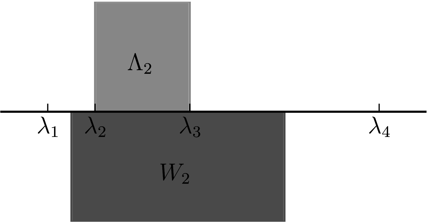
Examples
Undermentioned examples are made by Raymond Nung-Sing Sze.
Unitary matrices
1. Consider a diagonal unitary matrix $U_5 = \text{diag} (\{e^{2k \pi i/5}\}_{k=1}^5)$. The blue line represents the numerical range $\Lambda_1(U_5) = W(U_5)$ and the grey figure the real numerical shadow of $U_5$. The red polygon inside is $\Lambda_2(U_5)$. 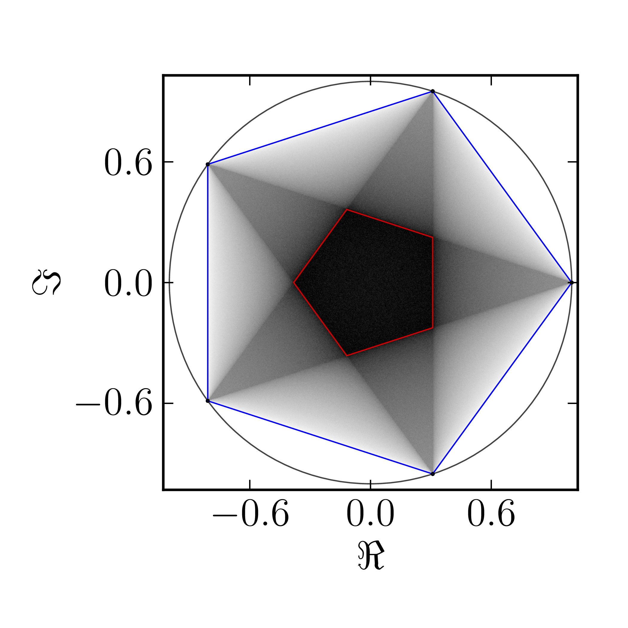
2. Consider a diagonal unitary matrix $U_7 = \text{diag} (\{e^{2k \pi i /7}\}_{k=1}^7)$. The blue line represents the numerical range $\Lambda_1(U_7) = W(U_7)$ and the grey figure the real numerical shadow of $U_7$. The red polygon inside is higher $2$-rank numerical range $\Lambda_2(U_7)$ and the green polygon is higher $3$-rank numerical range $\Lambda_3(U_7)$. 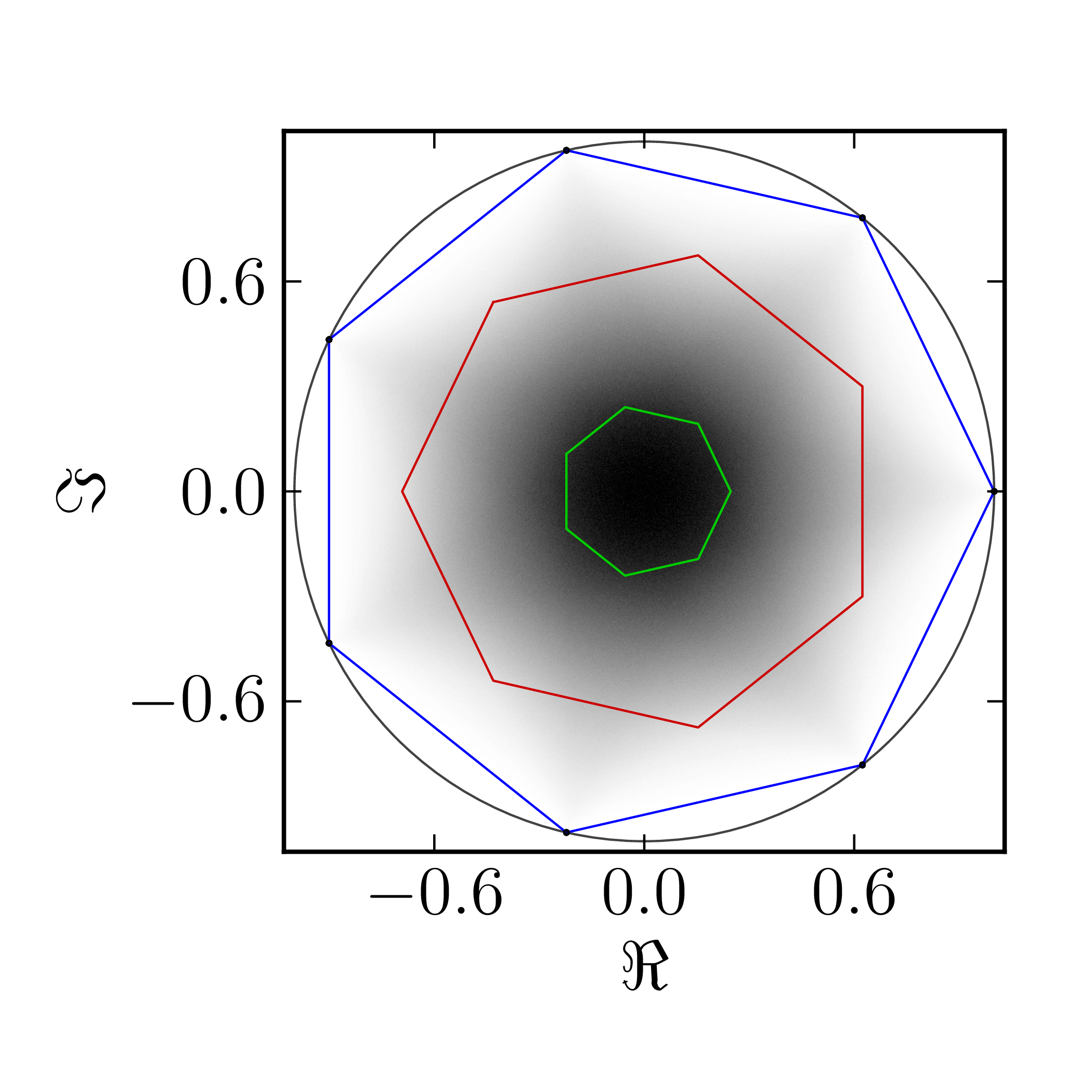
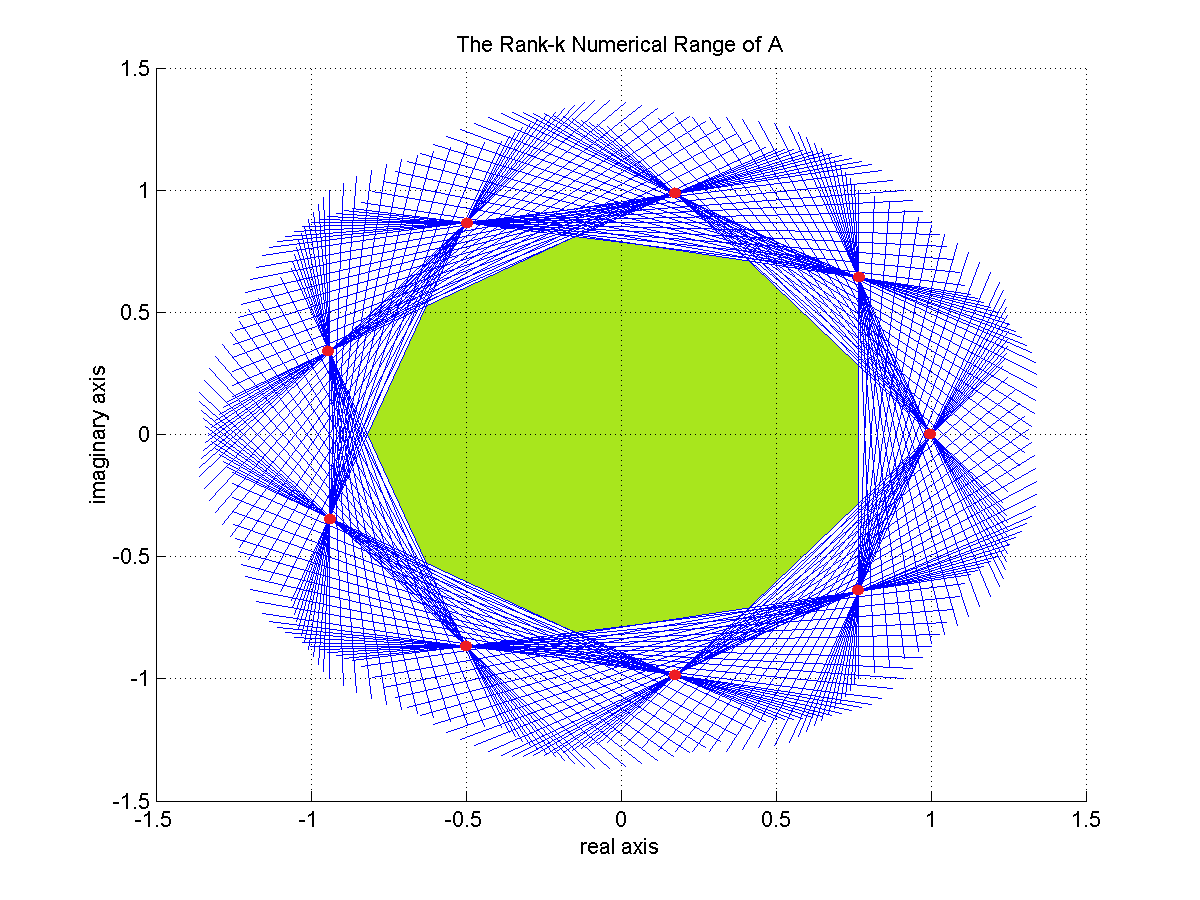
3. Consider a diagonal unitary matrix $A= \text{diag}(\{e^{2k \pi i /9}\}_{k=1}^9)$. The first picture represents $\Lambda_1(A) = W(A)$ classical numerical range of $A$ whereas the second picture represents higher $2$-rank numerical range $\Lambda_2(A)$. 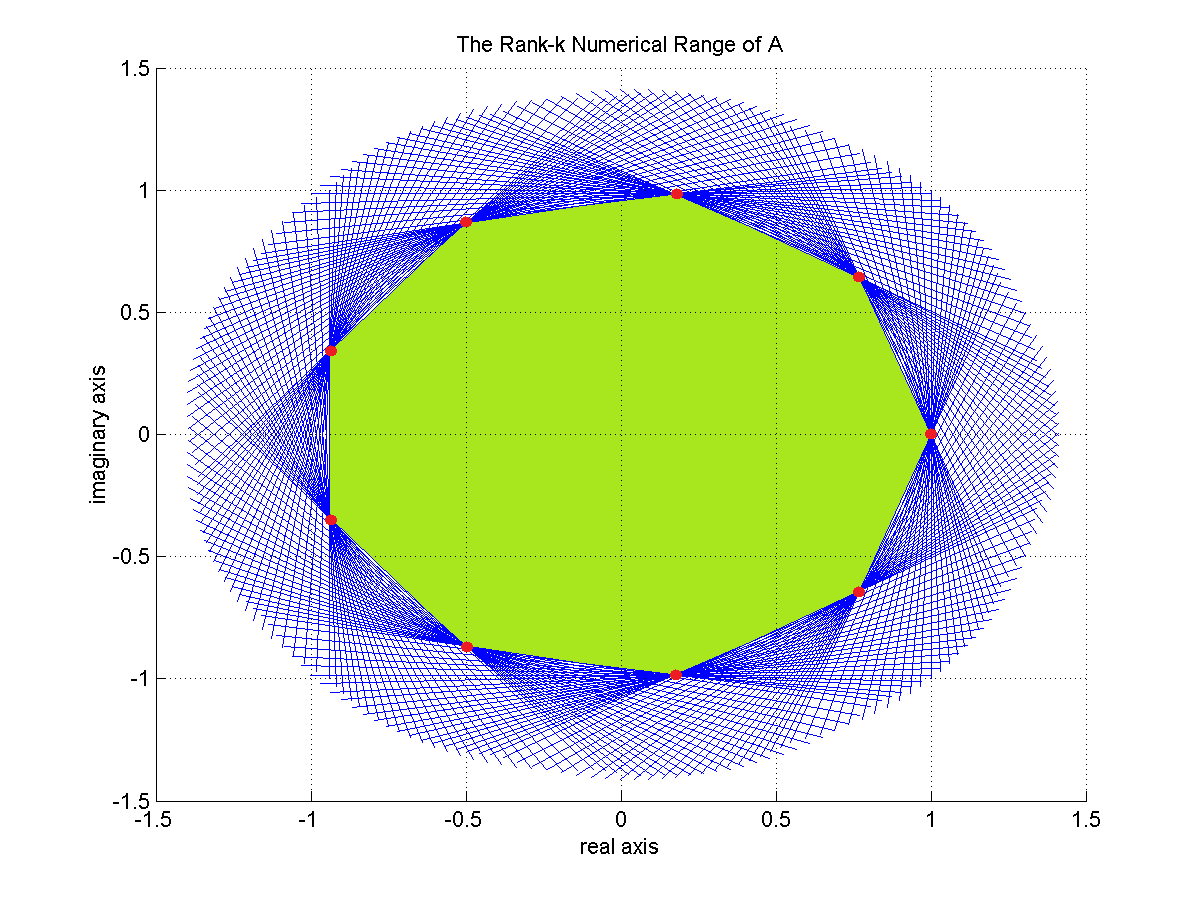
Non-normal matrices
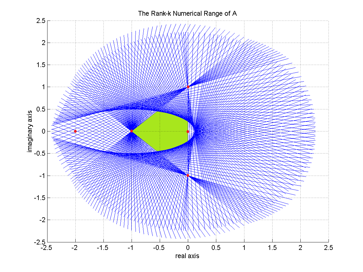
Let
$A=\begin{pmatrix} \ii & 0 & 0 & 0 & 0\newline 0 & -\ii & 0 & 0 & 0\newline 0 & 0 & -1 & 0 & 0\newline 0 & 0 & 0 & -2 & 1\newline 0 & 0 & 0 & 0 & 0 \end{pmatrix}$
will be non-normal matrix. Its numerical range is given by the first picture and higher $2$-rank numerical range is presented on the second picture. 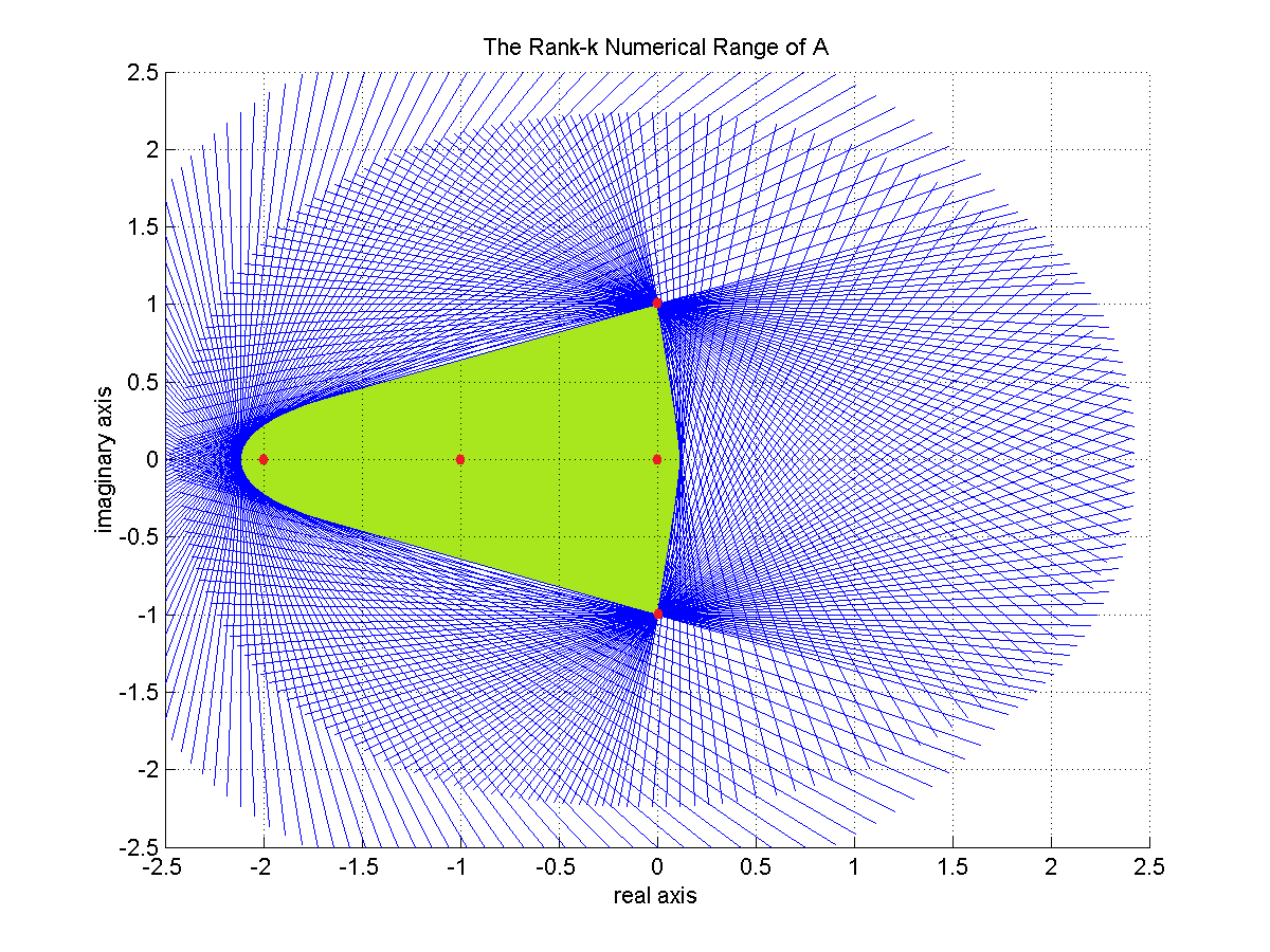
References
- [1]M. D. Choi, J. A. Holbrook, D. W. Kribs, and K. Życzkowski, “Higher-rank numerical ranges of unitary and normal matrices,” Operators and Matrices, vol. 1, pp. 409–426, 2007, [Online]. Available at: https://www.semanticscholar.org/paper/HIGHER-RANK-NUMERICAL-RANGES-OF-UNITARY-AND-NORMAL-Choi-Holbrook/5b13b6b5a92ce54bbf1699375a3ba26cbceb90ae.
- [2]H. J. Woerdeman, “The higher rank numerical range is convex,” Linear and Multilinear Algebra, vol. 56, no. 1-2, pp. 65–67, 2008, [Online]. Available at: https://www.tandfonline.com/doi/abs/10.1080/03081080701352211.
- [3]C. K. Li, Y. T. Poon, and N. S. Sze, “Condition for the higher rank numerical range to be non-empty,” Linear and Multilinear Algebra, vol. 57, no. 4, pp. 365–368, 2009, [Online]. Available at: https://www.tandfonline.com/doi/abs/10.1080/03081080701786384.
- [4]H.-L. Gau, C.-K. Li, and P. Y. Wu, “Higher-rank numerical ranges and dilations,” Journal of Operator Theory, vol. 0, pp. 181–189, 2010, [Online]. Available at: https://www.jstor.org/stable/24715918.
- [5]M.-T. Chien, C.-K. Li, and H. Nakazato, “The diameter and width of higher rank numerical ranges,” Linear and Multilinear Algebra, vol. 0, pp. 1–17, 2020, [Online]. Available at: https://www.tandfonline.com/doi/abs/10.1080/03081087.2019.1710105.
- [6]J. Holbrook, N. Mudalige, M. Newman, and R. Pereira, “Bounds on polygons of higher rank numerical ranges,” Linear Algebra and its Applications, vol. 474, pp. 230–242, 2015, [Online]. Available at: https://www.sciencedirect.com/science/article/pii/S0024379515000166.
- [7]M. D. Choi, D. W. Kribs, and K. Życzkowski, “Higher-rank numerical ranges and compression problems,” Linear algebra and its applications, vol. 418, no. 2, pp. 828–839, 2006, [Online]. Available at: https://arxiv.org/abs/math/0511278.
- [8]M. D. Choi, M. Giesinger, J. A. Holbrook, and D. W. Kribs, “Geometry of higher-rank numerical ranges,” Linear and Multilinear Algebra, vol. 56, no. 1-2, pp. 53–64, 2008, [Online]. Available at: https://www.tandfonline.com/doi/abs/10.1080/03081080701336545.
- [9]C. K. Li and N. S. Sze, “Canonical forms, higher rank numerical ranges, totally isotropic subspaces, and matrix equations,” Proceedings of the American Mathematical Society, vol. 136, no. 9, pp. 3013–3023, 2008, [Online]. Available at: https://www.ams.org/journals/proc/2008-136-09/S0002-9939-08-09536-1/.
- [10]M. Argerami and S. Mustafa, “Higher rank numerical ranges of Jordan-like matrices,” Linear and Multilinear Algebra, vol. 0, pp. 1–20, 2019, [Online]. Available at: https://www.tandfonline.com/doi/abs/10.1080/03081087.2019.1684873?journalCode=glma20.
- [11]M. Adam, A. Aretaki, and I. M. Spitkovsky, “Elliptical higher rank numerical range of some Toeplitz matrices,” Linear Algebra and its Applications, vol. 549, pp. 256–275, 2018, [Online]. Available at: https://www.sciencedirect.com/science/article/pii/S0024379518301344.