Joint numerical range

Definition

Consider $k$ Hermitian matrices $A_1,\ldots,A_k$ of dimension $d d$. Their joint numerical range (JNR)$L(A_1,,A_k)$ is defined as $L(A_1,\ldots,A_k) = \left\{ \left( \Tr \rho A_1,\ldots, \Tr \rho A_k \right): \rho \in \Omega_d \right\}.$ Due to taking all mixed states the joint numerical range is a convex body in a $k$-dimensional space. More information about convexity of joint numerical range we can find in [1].

Kippenhahn Theorem’s for joint numerical range

An algebraic curve has been associated with the numerical range and has been studied from the 1930s on [2]. Let $\1$ denote the $d\times d$ identity matrix, \[ p(x)=( x_0 \1 + x_1 A_1

• • x_n A_n ), \] and consider the complex projective hypersurface \[ (p)=\{x^n p(x) = 0 \}. \] It was shown that the eigenvalues of $A_1+ A_2$ are the foci of the affine curve of real points \[ T=\{ y_1+y_2 y_1,y_2,(1:y_1:y_2) (p)^\}. \] Kippenhahn recognized the meaning of the convex hull of $T$.

Theorem

The numerical range of $A_1+\ii A_2$ is the convex hull of $T$, in other words, $W(A_1+\ii A_2)=\text{conv}(T)$.

Let we denote $T_i$ as the semi-algebraic set \[ T_i = \{ (y_1,,y_n) (ⁿ⁾ (1:y_1::y_n)(X_i^)_ \}, i=1,,r \] and $(X^{}_i)_{\text{reg}}$ as the set of the regular points of the dual variety $X^$.

Theorem

The joint numerical range $W$ is the convex hull of the Euclidean closure of $T_1\cup\cdots\cup T_r$, in other words, $W = (T_1T_r)$.

Classification of JNRs

Two qutrit matrices

This classification comes from [3]. Consider two Hermitian matrices $A_1$ and $A_2$ of size $3 \times 3$. Then there are four possible shapes of the JNRs

• An oval–object without any flat parts, the boundary is a sextic curve.

• Object with one flat part, a convex hull of a quatric curve.

• Convex hull of an ellipse and an outside point, which has two flat parts on the boundary.

• A triangle (when $A_1$ and $A_2$ commute). This can be further degenerated.

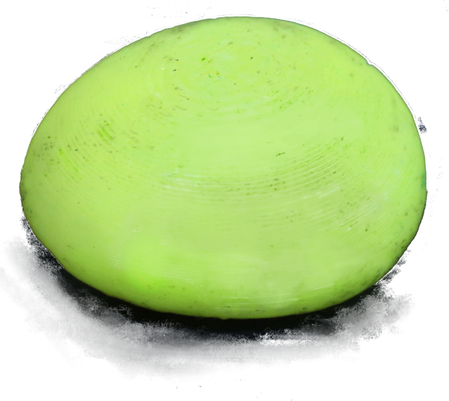
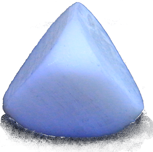
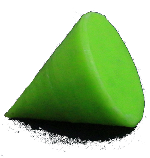
Three qutrit matrices

This classification is taken from [4] (see for details). Such JNRs must obey the following rules

1. In this case we may restrict ourselves to only pure states.
2. Any flat part in the boundary is the image of the Bloch sphere - two-dimensional subspace of a the sapce of $3 \times 3$ Hermitian matrices without corner points for

all configurations of Figure 2. We are unaware of earli

1. Two two-dimensional subspaces must share a common point, hence all flat parts are mutually connected.
2. Convex geometry of a three-dimensional Euclidean space supports up to four mutually intersecting ellipses.
3. If three ellipses are present in the boundary, the geometry does not allow for existence of any additional segment.
4. If two segments are present in the boundary, there exist an infinite number o other segments.

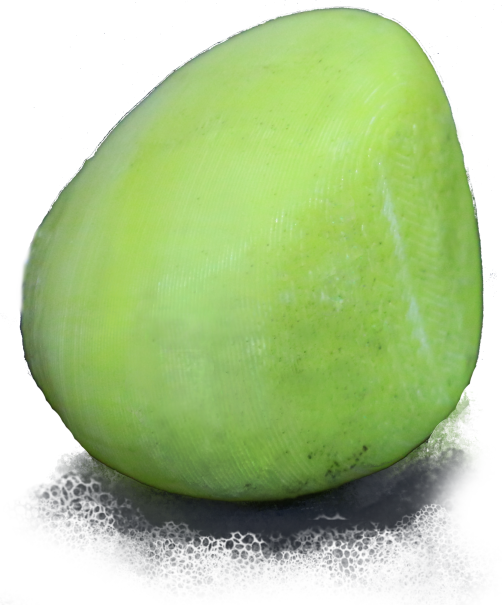
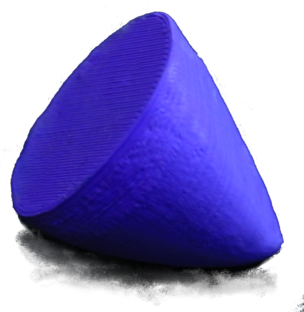
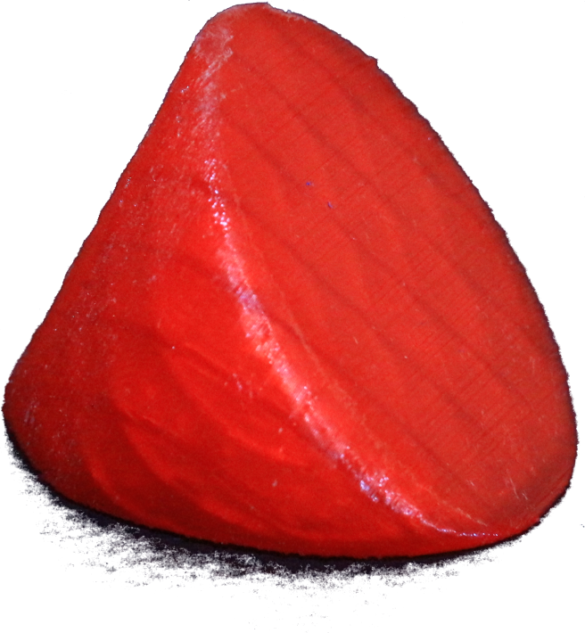
All configurations permitted by these rules are realized. Let us denote by $e$ the number of ellipses in the boundary and by $s$ the number of segments. There exists object with [5]:

• no flat parts in boundary at all $e=0$, $s=0$,
• one segment in the boundary $e=0$, $s=1$,
• one ellipse in the boundary $e=1$, $s=0$,
• one ellipse and a segment $e=1$, $s=1$,
• two ellipses in the boundry $e=2$, $s=0$,
• two ellipses and a segment $e=2$, $s=1$,
• three ellipses $e=3$, $s=0$,
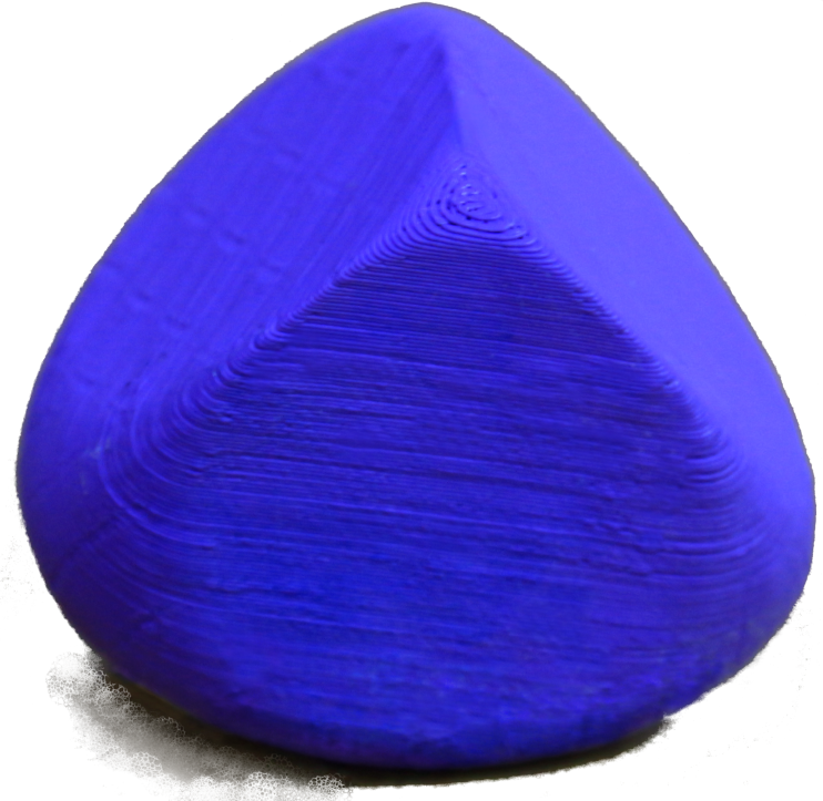
• four ellipses $e=4$, $s=0$,

Additionally in the qutrit case, if there exist of the JNR, the following configurations are possible:

• JNR is the convex hull of an ellipsoid and a point outside the ellipsoid, $e=0$, $s=\infty$,
• JNR is the convex hull of an ellipse and a point outside the affine hull of the ellipse, $e=1$, $s=\infty$,

Application

An example application of numerical range can be found in [6], [7], [2].

References

1. [1]C.-K. Li, Y.-T. Poon, and Y.-S. Wang, “Joint numerical ranges and communtativity of matrices,” arXiv preprint arXiv:2002.02768, vol. 0, 2020, [Online]. Available at: https://arxiv.org/abs/2002.02768.
   https://arxiv.org/abs/2002.02768
2. [2]D. Plaumann, R. Sinn, and S. Weis, “Kippenhahn’s Theorem for joint numerical ranges and quantum states,” arXiv preprint arXiv:1907.04768, vol. 0, 2019, [Online]. Available at: https://arxiv.org/abs/1907.04768.
   https://arxiv.org/abs/1907.04768
3. [3]D. S. Keeler, L. Rodman, and I. M. Spitkovsky, “The numerical range of 3x3 matrices,” Linear Algebra and its Applications, vol. 252, no. 1-3, pp. 115–139, 1997, [Online]. Available at: https://dx.doi.org/10.1016/0024-3795(95)00674-5.
   https://dx.doi.org/10.1016/0024-3795(95)00674-5
4. [4]K. Szymański, S. Weis, and K. Życzkowski, “Classification of joint numerical ranges of three hermitian matrices of size three,” Linear Algebra and its Applications, vol. 0, 2017, [Online]. Available at: https://www.sciencedirect.com/science/article/pii/S0024379517306456.
   https://www.sciencedirect.com/science/article/pii/S0024379517306456
5. [5]J. Xie et al., “Observing geometry of quantum states in a three-level system,” arXiv preprint arXiv:1909.05463, vol. 0, 2019, [Online]. Available at: https://arxiv.org/abs/1909.05463.
   https://arxiv.org/abs/1909.05463
6. [6]K. J. Szymański and K. Życzkowski, “Geometric and algebraic origins of additive uncertainty relations,” Journal of Physics A: Mathematical and Theoretical, vol. 0, 2019, [Online]. Available at: https://iopscience.iop.org/article/10.1088/1751-8121/ab4543/meta.
   https://iopscience.iop.org/article/10.1088/1751-8121/ab4543/meta
7. [7]J. Czartowski, K. Szymański, B. Gardas, Y. V. Fyodorov, and K. Życzkowski, “Separability gap and large-deviation entanglement criterion,” Physical Review A, vol. 100, no. 4, p. 042326, 2019, [Online]. Available at: https://journals.aps.org/pra/abstract/10.1103/PhysRevA.100.042326.
   https://journals.aps.org/pra/abstract/10.1103/PhysRevA.100.042326